On Feb 22, 2018, an article titled Identifying Medical Diagnoses and Treatable Diseases by Image-Based Deep Learning appeared in the front cover of the Cell Magazine.
Cell magazine publishes findings of unusual significance in any area of experimental biology, including cell biology, molecular biology, neuroscience, immunology, virology and microbiology, cancer, human genetics, systems biology, signaling, and disease mechanisms and therapeutics.
The authors have generously made the data and the code publicly available for further research. In this article, I will explain my successful attempt to recreate the results and explain my own implementation.
I have written this article for three different set of audiences:
1. General public who are interested in the application of AI for medical diagnosis.
2. Ophthalmologists who want to understand how AI can be used in their practice.
3. Machine learning students and new practitioners who want to learn how to implement such a system step by step.
A high level overview of what will be covered is listed below in the table of contents.
Table of Contents
Part 1 — Background and Overview
- Optical coherence tomography (OCT) and eye diseases
- Normal Eye Retina (NORMAL)
- Choroidal neovascularization (CNV)
- Diabetic Macular Edema (DME)
- Drusen (DRUSEN)
- Teaching humans to interpret OCT images for eye diseases
- Teaching computers to interpret OCT images for eye diseases — Algorithmic Approach
- Teaching computers to interpret OCT images for eye diseases — Deep Neural Networks
Part 2 — Implementation: Train the model
- Introduction
- Selection and Installation of Deep Learning Hardware and Software
- Download the data and organize
- Import required Python modules
- Setup the training and test image data generators
- Load InceptionV3 and attach new layers at the top
- Compile the model
- Fit the model with data and save the best model during training
- Monitor the training and plot the results
Part 3 — Implementation: Evaluate the Model
- Introduction
- Import required Python modules
- Load the saved best model
- Evaluate the model for a small set of images
- Write utility functions to get predictions for one image at a time
- Implement grad_CAM function to create occlusion maps
- Make prediction for a single image and create an occlusion map
- Make predictions for multiple images and create occlusion maps for misclassified images
Part 4: Summary and Download links
Clickable table of contents below:
Part 1 – Background and Overview
Optical coherence tomography (OCT) and eye diseases
Optical coherence tomography (OCT) is an imaging technique that uses coherent light to capture high resolution images of biological tissues. OCT is heavily used by ophthalmologists to obtain high resolution images of the eye retina. Retina of the eye functions much more like a film in a camera. OCT images can be used to diagnose many retina related eyes diseases. Three eye diseases of particular interest are listed below:
- Choroidal neovascularization (CNV)
- Macular Edema (DME)
- Drusen (DRUSEN)
The following picture shows the anatomy of the eye:

Normal Eye Retina (NORMAL)
The following picture shows OCT image of an normal retina.

Choroidal neovascularization (CNV)

Choroidal neovascularization (CNV) is the creation of new blood vessels in the choroid layer of the eye. CNV can create a sudden deterioration of central vision, noticeable within a few weeks. Other symptoms which can occur include color disturbances, and distortions in which straight lines appears wavy.
Diabetic Macular Edema (DME)

Diabetic Macular Edema (DME) occurs when fluid and protein deposits collect on or under the macula of the eye (a yellow central area of the retina) and causes it to thicken and swell (edema). The swelling may distort a person’s central vision, because the macula holds tightly packed cones that provide sharp, clear, central vision to enable a person to see detail, form, and color that is directly in the centre of the field of view.
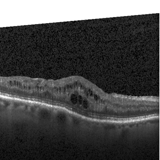
Drusen (DRUSEN)

Drusen are yellow deposits under the retina. Drusen are made up of lipids, a fatty protein. There are different kinds of drusen. “Hard” drusen are small, distinct and far away from one another. This type of drusen may not cause vision problems for a long time, if at all.
Teaching humans to interpret OCT images for eye diseases
How would you train humans to identify the four classes of eye conditions (CNV, DME, DRUSEN, or NORMAL) from OCT images? First, you would collect a large number of pictures (say 100) of each condition and organize them. You would then label the images (CNV, DME, DRUSEN, or NORMAL) and annotate few image of each condition to show where to look for abnormalities.
You would then show the examples, help the human to identify critical features in the image and help them classify the pictures into one of the four conditions (we’ll call them classes from now on). At the end of the training, you would them show pictures randomly and check if they can classify the images correctly.
Teaching computers to interpret OCT images for eye diseases – Algorithmic Approach
Traditionally, algorithmic approach is used for image analysis. In this method, experts study the images and identify key features in the image. Then use statistical methods to identify key features , and finally classify the whole image. This method requires many experts, lot of time and is expensive.
Teaching computers to interpret OCT images for eye diseases – Deep Neural Networks
The recent advances in machine learning using feedforward deep neural networks with multiple convolutional layers makes the training computers easy for such tasks. It is shown that the performance of neural networks increases with increase in the amount of training data available. The amount of published OCT images is limited although the authors of the papers have released 100,000 images. The neural networks tends to work better with millions of images.
The key idea is to use a neural network that has already been trained to detect 1,000 classes of images (dogs, cats, cars etc) with millions of images. One such dataset is ImageNet that consists of 14 million images. A ImageNet trained Keras model of GoogleNet (Inception v3) is already available here.
A model implements a particular neural network topology consisting of many layers. In simpler terms, the images are fed to the bottom layer (input) of the model and the topmost layer produces the output.
First, we remove the fully connected top layers (close to the output) of the model that classifies the images to 1,000 classes. Let us call this model without the top layers, the base model. We then attach few new layers to the top that classify the images into four classes of our interest: 1. CNV, 2.DME, 3. DRUSEN, 4. NORMAL.
The layers in the base model are locked and made not trainable. The base model parameters (also called weights) are not updated during training. The new updated model is trained with 100,000 OCT images with additional 1,000 images used for validation. This method is called the transfer learning. I have fully trained Keras model that achieves 94% validation accuracy and is available for anyone to download and use.
Along with the model, a simple Python method to produce occlusion maps is also available. Occlusion map shows which part of the image did the neural network paid more attention to make the decision to classify the image. One such occlusion map for DRUSEN is shown below.

The Gradient-weighted Class Activation Mapping (Grad-CAM) technique is being used to produce these occlusion maps.
Some of the benefits of using neural networks for these tasks are as follows:
- The model is easy to train with existing data and retrain when new data is made available.
- The model can classify new unseen images under less than a second. The model can be be embedded in the OCT machines and also can be made available as a smartphone app or a web app.
- Occlusion maps help us determine which part (which features) of the image played a key role in classifying the image. These maps can be used for training humans to read the OCTs.
- Using Generative adversarial network (GAN) techniques a large number synthetic image samples can be generated and used for training humans and new neural networks.
Rest of the article focuses on the step by step tutorial, annotated code samples to help you train your own model and achieve the same results of the original paper.
Part 2 – Implementation: Train the model
Introduction
In this part, I will provide step by step tutorials, annotated code samples to help you train your own model.
This part will cover the following:
- Selection and installation of deep learning hardware and software.
- Download the data and organize.
- Writing code to train the model.
- Next part will cover evaluation of the model accuracy and occlusion maps.
The implementation is available eyediseases-AI-keras-imagenet-inception. Use Train.ipynb under jupyter notebook.
Selection and Installation of Deep Learning Hardware and Software
A general purpose computer or a server is not well suited for training a deep neural network that is capable of processing 100,000 images. For training purposes, I have use a customized low cost hardware with the following specifications:
- Intel – Core i3-6100 3.7GHz Processor
- ASUS – Z270F GAMING 3X ATX LGA1151 Motherboard
- Corsair 16GB – Vengeance LPX 8GB (8GBx2) DDR4-2400
- GeForce GTX 1060 6GB Mini ITX OC Graphic Card
- Antec power supply 600 Watts
- Antec Cabinet (GX200)
- Samsung- SSD PLUS 2 x 240GB 2.5″ Solid State Drive
The detailed parts list is also available at PC Part Picker.
You can learn about how to build your own deep learning hardware from this wonderful article: Build a Deep Learning Rig for $800. Same author has published an article Ubuntu + Deep Learning Software Installation Guide that you will also find it useful.
Alternatively, you could use a GPU enabled Amazon Web Service (AWS) instance. The low end typically costs $0.90/hour. For the price of one month running costs, you can build your own Deep Learning Machine.
The good people at Cache Technologies, Bangalore helped me build the machine and test it.
For rest of the software, I have used the following:
Download the data and organize
Visit Labeled Optical Coherence Tomography (OCT) and Chest X-Ray Images for Classification page and download OCT2017.tar.gz (3.4GB).
Dataset of validated OCT and Chest X-Ray images described and analyzed in “Deep learning-based classification and referral of treatable human diseases”. The OCT Images are split into a training set and a testing set of independent patients. OCT Images are labeled as (disease)-(randomized patient ID)-(image number by this patient) and split into 4 directories: CNV, DME, DRUSEN, and NORMAL.
Extract the tar file using the following command:
% tar xvfz OCT2017.tar.gz
This should create the OCT2017 folder with following sub folders: test and train. Both test and train will have sub folders named: CNV, DME, DRUSEN, and NORMAL. These bottom most folders have the gray scale OCT images.
Create another folder named eval under OCT2017. Create the required sub folders CNV, DME, DRUSEN, and NORMAL. Move few (100 images) from test and train folders to the correct eval folders finally use to evaluate the model.
Import required Python modules
The analysis code is written in python running inside Jupyter notebook. You can copy paste the code from below to cells in order and press Shift + Enter to execute the cell.
First step is to import the required modules:
import keras
from keras.preprocessing.image import ImageDataGenerator
from keras.applications.inception_v3 import InceptionV3
from keras.layers import Dense, GlobalAveragePooling2D
from keras.models import Model
from keras import optimizers
import matplotlib.pyplot as plt
%matplotlib inline
ImageGenerator is used to rescale the image values and will be used yield batch of images during training.
InceptionV3 is the keras implementation of Inception V3 model and is made available with imagenet weights.
GlobalAveragePooling2D and Dense will be the new set of layers that we will add to the top of the InceptionV3 model after removing existing fully connected top layers.
Setup the training and test image data generators
train_datagen = ImageDataGenerator(rescale=1./255)
test_datagen  = ImageDataGenerator(rescale=1./255)
train_dir     = '../OCT2017/train/'
test_dir      = '../OCT2017/test/'
train_generator = train_datagen.flow_from_directory(
                    train_dir, target_size=(299, 299),
                    batch_size=128, class_mode='categorical')
test_generator = test_datagen.flow_from_directory(
                   test_dir, target_size=(299, 299),
                   batch_size=128, class_mode='categorical')
When you read the image file, the values of the pixels are in grey scale ranging from 0 to 255. Rescaling reduces the values to the range 0 to 1.0. It is important to remember this rescaling value during evaluation and making predictions.
The train_generator and test_generator yields 128 images in each batch of size 299×299. The number of images per batch is a function of how much memory your GPU and the main system have. The original authors have used 1,000 images per batch. The 299×299 image size is the input size required for Inception V3 model. Read more about ImageDataGenerator here.
The class_mode is set to categorial as we need the output to belong to 4 classes (CNV, DME, DRUSEN, and NORMAL).
Load InceptionV3 and attach new layers at the top
# create the base pre-trained model
base_model = InceptionV3(weights='imagenet',
                include_top=False)
# Get the output layer from the pre-trained Inception V3 model
x = base_model.output

# Now, add new layers that will be trained with our data
# These layers will be randomly initialized
x = GlobalAveragePooling2D()(x)
x = Dense(64, activation='relu')(x)
predictions = Dense(4, activation='softmax')(x)

# Get the final Model to train
model = Model(inputs=base_model.input, outputs=predictions)

# Freeze the layers from the original base model so that we don't update the weights
for layer in base_model.layers:
    layer.trainable = False
First, we load the InceptionV3 model with pre-trained weights for imagenet. Set include_top=False to exclude the fully-connected layer at the top of the network that outputs 1,000 classes. Instead, we will be adding our own fully connected layer that will output 4 classes using softmax.
Next, add three layers (GlobalAveragePooling2D, Dense, Dense with softmax) to the top. We use GlobalAveragePooling2D instead of a fully connected (i.e Dense) to process the output of the InceptionV3 base model. This helps in avoiding overfitting and reducing the number of parameters in the final model. The last Dense model has 4 units corresponding to the number of output classes : CNV, DME, DRUSEN, and NORMAL.
Finally, make the original InceptionV3 base model not trainable, that is, freeze the network. These weights have been already trained with imagenet. If you make these trainable, the layer parameters (weights) will get updated with large changes during the initial training making them forget the original learning. Locking the layers also makes the training faster as during back propagation these layer parameters need not be computed and updated.
Compile the model
adam = optimizers.adam(lr=0.001)
# Compile the new model
model.compile(optimizer=adam,
  loss='categorical_crossentropy', metrics=['accuracy'])
Choose adam as the optimizer with learning rate set to 0.001. We are interested in minimizing loss for categorial cross entropy (meaning many categories: 4 to be specific). Train, test accuracy, and losses are the metrics that we interested in.
Fit the model with data and save the best model during training
# Setup a callback to save the best model
callbacks = [keras.callbacks.ModelCheckpoint(
    'model.{epoch:02d}-{val_acc:.2f}.hdf5',
     monitor='val_acc', verbose=1,
     save_best_only=True, mode='max', period=1)]

# Fit the data and output the history
history = model.fit_generator(train_generator,
  verbose=1, steps_per_epoch=len(train_generator),
  epochs=100, validation_data=test_generator,
  validation_steps=len(test_generator), callbacks=callbacks)
You want to save the best performing models during training. The best performing model is one which provides the highest validation accuracy. The output file, for example would be the following:
model.03-0.94.hdf5
03 is the epoch number and 0.94 is the validation accuracy.
To fit the data, specify the number of epochs, meaning the number of times the model will see the whole dataset. The steps_per_epoch is the number of batches of data that the model will see in one epoch. Set this to the total number of batches that the data generator will yield.
Monitor the training and plot the results
def plot_history(history):
    acc = history.history['acc']
    val_acc = history.history['val_acc']
    loss = history.history['loss']
    val_loss = history.history['val_loss']

    epochs = range(1, len(acc) + 1)

    plt.figure()
    plt.title('Training and validation accuracy')
    plt.plot(epochs, acc, 'bo', label='Training acc')
    plt.plot(epochs, val_acc, 'b', color='red', \
       label='Validation acc')
    plt.legend()
    plt.show()

    plt.figure()
    plt.title('Training and validation loss')
    plt.plot(epochs, loss, 'bo', label='Training loss')
    plt.plot(epochs, val_loss, 'b', color='red', \
       label='Validation loss')
    plt.legend()
    plt.show()
    return acc, val_acc, loss, val_loss

acc, val_acc, loss, val_loss = plot_history(history)
If all goes well, you should have a set of saved models, and two graphs showing the accuracy (training and validation) and loss (training and validation).


During the training, monitoring of GPU, CPU, and memory utilization is critical. In my earlier attempts, GPU ran out of memory!


Part 3 – Implementation: Evaluate the Model
Introduction
In this part, I’ll outline how to evaluate the trained model and make predictions using new set of images.
The implementation is available at GitHub: eyediseases-AI-keras-imagenet-inception. Use Evaluate.ipynb under jupyter notebook.
Import required Python modules
The analysis code is written in python running inside Jupyter notebook. You can copy paste the code from below to cells in order and press Shift + Enter to execute the cell.
First step is to import the required modules:
import os
import numpy as np

import keras
from keras.preprocessing.image import ImageDataGenerator, \
 load_img, img_to_array

from keras.models import load_model
from keras import backend as K

from io import BytesIO
from PIL import Image
import cv2

import matplotlib.pyplot as plt
import matplotlib.image as mpimg
from matplotlib import colors

import requests

K.set_learning_phase(0) #set the learning phase to not training
We will be using OpenCV (cv2) for generating occlusion maps. requests library allow us to feed image referenced by an URL. It is important to set the learning phase as not training (0) to avoid errors from the keras library.
Load the saved best model
model = load_model('model.03-0.94.hdf5')
Evaluate the model for a small set of images
# Set the image generator
eval_datagen = ImageDataGenerator(rescale=1./255)
eval_dir = '../OCT2017/eval'

eval_generator = eval_datagen.flow_from_directory( \
  eval_dir, target_size=(299, 299), batch_size=32, \
  class_mode='categorical')
# Evaluate the model for a small set of images
loss = model.evaluate_generator(eval_generator, steps=10)
out = {}
for index, name in enumerate(model.metrics_names):
 print(name, loss[index])
Write utility functions to get predictions for one image at a time
# Utility functions
classes = ['CNV', 'DME', 'DRUSEN', 'NORMAL']
# Preprocess the input
# Rescale the values to the same range that was
# used during training
def preprocess_input(x):
    x = img_to_array(x) / 255.
    return np.expand_dims(x, axis=0)

# Prediction for an image path in the local directory
def predict_from_image_path(image_path):
    return predict_image(load_img(image_path,
       target_size=(299, 299)))

# Prediction for an image URL path
def predict_from_image_url(image_url):
    res = requests.get(image_url)
    im = Image.open(BytesIO(res.content))
    return predict_from_image_path(im.fp)

# Predict an image
def predict_image(im):
    x = preprocess_input(im)
    pred = np.argmax(model.predict(x))
    return pred, classes[pred]
Implement grad_CAM function to create occlusion maps
def grad_CAM(image_path):
    im = load_img(image_path, target_size=(299,299))
    x = preprocess_input(im)
    pred = model.predict(x)

    # Predicted class index
    index = np.argmax(pred)

    # Get the entry of the predicted class
    class_output = model.output[:, index]

    # The last convolution layer in Inception V3
    last_conv_layer = model.get_layer('conv2d_94')
    # Has 192 channels
    nmb_channels = last_conv_layer.output.shape[3]

    # Gradient of the predicted class with respect to
    # the output feature map of the
    # the convolution layer with 192 channels
    grads = K.gradients(class_output,  \
              last_conv_layer.output)[0]

    # Vector of shape (192,), where each entry is the mean intensity of the gradient over
    # a specific feature-map channel”
    pooled_grads = K.mean(grads, axis=(0, 1, 2))

    # Setup a function to extract the desired values
    iterate = K.function(model.inputs,
       [pooled_grads, last_conv_layer.output[0]])
    # Run the function to get the desired calues
    pooled_grads_value, conv_layer_output_value = \
         iterate([x])

    # Multiply each channel in the feature-map array by “how important this channel is” with regard to the
    # predicted class

    for i in range(nmb_channels):
        conv_layer_output_value[:, :, i] *=  \
               pooled_grads_value[i]

    # The channel-wise mean of the resulting feature map is the heatmap of the class activation.
    heatmap = np.mean(conv_layer_output_value, axis=-1)

    # Normalize the heatmap betwen 0 and 1 for visualization
    heatmap = np.maximum(heatmap, 0)
    heatmap /= np.max(heatmap)

    # Read the image again, now using cv2
    img = cv2.imread(image_path)
    # Size the heatmap to the size of the loaded image
    heatmap = cv2.resize(heatmap, (img.shape[1], \
                 img.shape[0]))
    # Convert to RGB
    heatmap = np.uint8(255 * heatmap)
    # Pseudocolor/false color a grayscale image using OpenCV’s predefined colormaps
    heatmap = cv2.applyColorMap(heatmap, cv2.COLORMAP_JET)

    # Superimpose the image with the required intensity
    superimposed_img = heatmap * 0.5 + img

    # Write the image
    plt.figure(figsize=(24,12))
    cv2.imwrite('./tmp.jpg', superimposed_img)
    plt.imshow(mpimg.imread('./tmp.jpg'))
    plt.show()
The above code was adapted from https://www.manning.com/books/deep-learning-with-python. This is a great book read!
Make prediction for a single image and create an occlusion map
predict_from_image_path('../OCT2017/eval/DRUSEN/DRUSEN-53018-1.jpeg')
grad_CAM('../OCT2017/eval/DRUSEN/DRUSEN-53018-1.jpeg')
The output should be as follows:
(2, 'DRUSEN')

The image shows which part of the image did the model look at to make the prediction.
Make predictions for multiple images and create occlusion maps for misclassified images
for i, c in enumerate(classes):
    folder = './simple/test/' + c + '/'
    count = 1
    for file in os.listdir(folder):
        if file.endswith('.jpeg') == True:
            image_path = folder + file
            p, class_name = predict_from_image_path(image_path)
            if p == i:
                print(file, p, class_name)
            else:
                print(file, p, class_name, \
                    '**INCORRECT PREDICTION**')
                grad_CAM(image_path)
        count = count +1
        if count == 100:
            continue
Here is an example of how DME was misclassified as DRUSEN output will look like:

The above picture shows how the model was confused between DME and DRUSEN. It payed attention more to the DRUSEN features instead of DME.
Part 4: Summary and download links
In this article, I have described three specific eye retinal diseases and how they can be identified from Optical coherence tomography (OCT) images along with normal eye retina.
Using transfer learning technique, I show how Keras imagenet pretrained InceptionV3 model can be trained using a large number of OCT images. We remove the top layers, add our own fully connected layers, and lock the base model to complete the training.
We save the best models during training using Keras callbacks. Using metrics we analyze the progress of the training.
Using the best saved model, we did predictions for new images and use occlusion maps to better understand the model’s behavior.
Annotated source code (Jupyter notebook and Python) is available at GitHub: eyediseases-AI-keras-imagenet-inception. The trained model with 94% validation accuracy can be downloaded from here (84MB file!).
I hope you liked this article! Please share your experiences and feedback to this make article better.
Update – Follow up article!
Please read the second article in the series with improved accuracy and fast training:
- Best performing model at 99.10% accuracy
- Repeatable accuracy at >98%
- Each epoch take around 1.5 minutes compared to 12 minutes as before.
- Requires only 50 epochs (75 minutes) when compared to 500 epochs (100 hours) to achieve convergence.
- Model size has reduced from 84MB to 1.7MB
Leave a Reply
You must be logged in to post a comment.